Dec 13
Neural Networks via Information
Until this day, the theoretical mechanisms of learning with Deep Neural Network (DNN) are not well known. One remarkable contribution is the concept of Information Bottleneck (IB) presented by Naftali Tishby [1,2], who was a computer scientist and neuroscientist from the Hebrew University of Jerusalem. His theory claims to be a way to understand the impressive success of neural networks in a huge variety of applications. Hence, I’m presenting a general vision of DNN via information and creating my own experimental setup to check the IB.

How does information theory help us to better understand DNN?
Imagine a common problem of image classification of cats and dogs. A photo can be represented by a random variable X and the label by a random variable Y. If we want to create a machine that can classify correctly each image, we expect that it should be able to extract the important features to predict if the image is indeed from a dog or a cat. These important features of X to describe Y can be measured using the mutual information, I[X,Y]. This quantity measures the bits of information shared by X and Y.

However, the task of extracting and compressing the useful information of X to predict Y is not trivial, actually, it’s quite challenging, leading to the loss of useful information. In that context, DNN emerges as a strong competitor in finding the optimal characterization of the information subjected to the tradeoff between compression and prediction success. That’s the idea of the Information Bottleneck (IB).
Information Bottleneck and DNN
The power of the DNN lies inside the internal representation through the layers, actually, the neural network represents a Markov chain of successive representations of the input layer X → T_1 → T_2 → …→ T_n → Y [3]. As mentioned earlier the goal is to find the optimal representation T(X) that extracts the important features of X to predict Y, therefore, mutual information is an important tool that able us to measure information shared by 2 random variables with a joint distribution p(X,Y).

1. Mutual Information
Measures the amount of information shared by two random variables X and Y (the unit is usually in bits).
It's defined as

where

H[x] is our ignorance over X, as known as entropy, and H(X∣Y) is our ignorance of X given that we have Y, which is the conditional entropy. Once, we understand the idea of mutual information, we’re ready for the Data Processing Theorem.
2. The Data Processing Theorem
The theorem states that every irreversible transformation dissipates information.
X→ T_1 → Y → T_2 → Z, then, I[X,Y] ≥ I[X,Z].
For a Neural network

But we still did not answer how to find the optimal representation T(X). The minimal sufficient statistics might get us on the right path.
3. Minimal Sufficient Statistics
Minimal Sufficient Statistics is a function of X, S(X), that preserves all the information about the parameters of the distribution p(X,θ) (e.g. mean (μ) and standard deviation (σ) of a normal distribution). However, for our context, we can understand that as the function that compresses and transform the data without losing any information about Y.
The problem is that minimal sufficient statistics exist for only a subset of distributions (i.e exponential family), so it’s a very strong assumption to use in Machine Learning. Hence, we need to find a way to approximate the minimal sufficient statistics to capture as much as possible of I[X,Y]. In that context, we finally arrive at the Information Bottleneck.
4. Information Bottleneck
Let T be a parametrized transformation T = ϕ(X,θ), that can be a series of transformations T_1,T_2… We can choose T in a way that conserves more information of Y extracting only the relevant features of X, lending to the tradeoff between prediction and compression.

Therefore, the information bottleneck is a framework to find an approximation of the minimal sufficient statistics, whence, the optimal tradeoff between compression of X and prediction of Y.
An important remark is the relevance of Stochastic Gradient Descent (SGD), commonly used in DNN to estimate the parameters given a loss function. Tishby explores the SGD dynamics as a major way to achieve IB bound, which means the transformation T that obeys the tradeoff.
Now that we better understand the relationship between DNN and information bottleneck, we must check it with a simple neural network and simulated data.

Testing IB & DNN
For the numerical simulation, I opted to create a binary problem, as estimating mutual information for continuous variables can be difficult. Making a more robust estimate leads us to a more reliable result.
Therefore, I simulated data following Y = h( g( X ) + ϵ ), where X=(x_1,x_2,…,x_10) and x_i = {0,1} is a Bernoulli variable with p = 1/2, g a non-linear function and h a function to binarize the input, ϵ ∼ N(0,1) is a gaussian noise.

where

Resulting in a balanced dataset

To estimate the mutual information I used frequency as an approximation for the probabilities and defined some entropy properties.
Therefore, the mutual information of X and Y is I[X,Y] = 0.82, this is an important result since it's part of the Information Bottleneck (IB) bound. Now, we create a very simple Neural Network, with 3 layers and 3,2,1 neurons, respectively.
Once we created the neural network architecture, we need the output of each layer in all epochs. In this way, the data of each representation T_1, T_2 and T_3 through epochs is stored in activation_list.
Since the output from the layers is continuous, we need to discretize it in bins.
Now, we calculate the information plane ( I[X,Y] and I[T,Y]).
And plot the results.

Hence, it's clear that all the layers get closer to the information bottleneck bound over the epochs.
Other approaches
The information theory is a powerful mathematical structure to comprehend machine learning, in that context many different approaches are created to increase our understanding of learning. One notorious example is the Minimal Achievable Sufficient Statistic (MASS) Learning, which is a method to find minimal sufficient statistics, or optimal representations, following a similar framework of the information bottleneck, but well adapted to continuous variables [4]. The results have a competitive performance on supervised learning and uncertainty quantification benchmarks.
Acknowledgments
This project was developed for the course Information Systems Theory, Bayesian Inference and Machine Learning, conceived and taught by Prof. Renato Vicente.
The notebook for this article is available here.
References
[1] N. Tishby, Fernando C. Pereira, and W. Bialek, The information bottleneck method (1999), In Proceedings of the 37-th Annual Allerton Conference on Communication, Control and Comput- ing, 1999.
[2] Shwartz-Ziv, Ravid, and N. Tishby, Opening the Black Box of Deep Neural Networks via Information (2017), doi:10.48550/ARXIV.1703.00810.
[3] N. Tishby and N. Zaslavsky, Deep learning and the information bottleneck principle (2015), In Information Theory Workshop (ITW), 2015 IEEE, pages 1–5. IEEE, 2015.
[4] M. Cvitkovic and G. Koliander, Minimal Achievable Sufficient Statistic Learning (2019), Proceedings of the 36th International Conference on Machine Learning, PMLR 97:1465–1474, 2019.